
Chin J Plant Ecol ›› 2008, Vol. 32 ›› Issue (1): 152-160.DOI: 10.3773/j.issn.1005-264x.2008.01.017
• Research Articles • Previous Articles Next Articles
SONG Kai-Shan1( ), ZHANG Bai1, WANG Zong-Ming1, LIU Dian-Wei1, LIU Huan-Jun1,2
Received:2007-01-05
Accepted:2007-09-24
Online:2008-01-05
Published:2008-01-30
Contact:
SONG Kai-Shan
SONG Kai-Shan, ZHANG Bai, WANG Zong-Ming, LIU Dian-Wei, LIU Huan-Jun. SOYBEAN CHLOROPHYLL A CONCENTRATION ESTIMATION MODELS BASED ON WAVELET-TRANSFORMED, IN SITU COLLECTED, CANOPY HYPERSPECTRAL DATA[J]. Chin J Plant Ecol, 2008, 32(1): 152-160.
| 植被指数 Vegetation index | 植被指数采用的公式及波段 Formula and bands applied | 文献来源 References |
|---|---|---|
| 归一化植被指数 Normalized difference vegetation index (NDVI) | (R801-R670)/(R801+R670) | |
| 土壤调和植被指数 Soil-adjusted vegetation index (SAVI) | (1+L)×(R801-R670)/(R801+R670+L) | |
| 再归一植被指数 Renormalized difference vegetation index (RDVI) | RDVI=(R801-R670)/ | |
| 第二修正比值植被指数 Modified second ratio index (MSR) | MSRI=( |
Table 1 Vegetation indices evaluated in the present study
| 植被指数 Vegetation index | 植被指数采用的公式及波段 Formula and bands applied | 文献来源 References |
|---|---|---|
| 归一化植被指数 Normalized difference vegetation index (NDVI) | (R801-R670)/(R801+R670) | |
| 土壤调和植被指数 Soil-adjusted vegetation index (SAVI) | (1+L)×(R801-R670)/(R801+R670+L) | |
| 再归一植被指数 Renormalized difference vegetation index (RDVI) | RDVI=(R801-R670)/ | |
| 第二修正比值植被指数 Modified second ratio index (MSR) | MSRI=( |
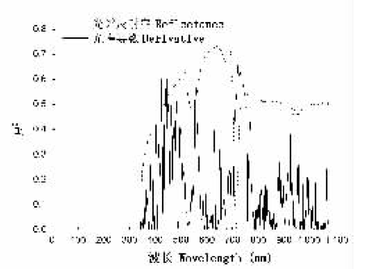
Fig.1 Coefficient of determination (R2) derived from a linear regression of reflectance and derivative against chlorophyll a concentration
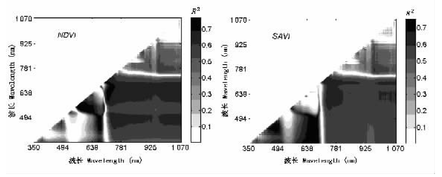
Fig.2 Coefficient of determination for all combinations of wavelength used for linear regression analysis of NDVI and SAVI against chlorophyll a concentration,respectively NDVI、SAVI: See Table 1
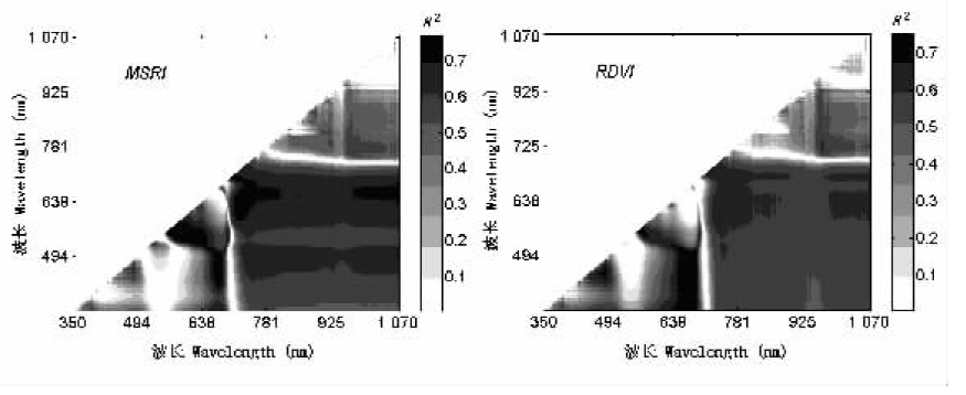
Fig.3 Coefficient of determination for all combinations of wavelength used for linear regression analysis of MSRI and RDVI against chlorophyll a concentration,respectively MSRI、RDVI: See Table 1
| 植被指数 Vegetation indices | 线性估算模型 Linear regression model (n=100) | 模型验证 Model validation (n=44) | ||||||
|---|---|---|---|---|---|---|---|---|
| 回归公式 Regression formula | R2 | RMSE (mg·g-1) | R2 | RMSE (mg·g-1) | ||||
| NDVI (441,223) | y=5.317x-3.223 | 0.782 | 0.168 | 0.754 | 0.173 | |||
| SAVI (502,32) | y=-20.621x+1.644 | 0.762 | 0.171 | 0.734 | 0.181 | |||
| RDVI (488,28) | y=-17.073 0x+1.757 8 | 0.759 | 0.172 | 0.722 | 0.189 | |||
| MSRI (257,128) | y=10.358 0x-9.512 9 | 0.769 | 0.170 | 0.731 | 0.182 | |||
| 植被指数 Vegetation indices | 非线性估算模型 Non-linear regression model (n=100) | 模型验证 Model validation (n=44) | ||||||
| 回归公式 Regression formula | R2 | RMSE (mg·g-1) | R2 | RMSE (mg·g-1) | ||||
| NDVI (441,223) | y=0.019e4.722x | 0.793 | 0.164 | 0.726 | 0.186 | |||
| SAVI (502,32) | y=2.077e-18.03x | 0.798 | 0.162 | 0.732 | 0.182 | |||
| RDVI (488,28) | y=1.851e-14.91x | 0.778 | 0.171 | 0.717 | 0.193 | |||
| MSRI (257,128) | y=0.880x5.81 | 0.805 | 0.158 | 0.747 | 0.176 | |||
Table 2 Linear and non-linear regression models based on optimum spectral vegetation indices against chlorophyll a concentration
| 植被指数 Vegetation indices | 线性估算模型 Linear regression model (n=100) | 模型验证 Model validation (n=44) | ||||||
|---|---|---|---|---|---|---|---|---|
| 回归公式 Regression formula | R2 | RMSE (mg·g-1) | R2 | RMSE (mg·g-1) | ||||
| NDVI (441,223) | y=5.317x-3.223 | 0.782 | 0.168 | 0.754 | 0.173 | |||
| SAVI (502,32) | y=-20.621x+1.644 | 0.762 | 0.171 | 0.734 | 0.181 | |||
| RDVI (488,28) | y=-17.073 0x+1.757 8 | 0.759 | 0.172 | 0.722 | 0.189 | |||
| MSRI (257,128) | y=10.358 0x-9.512 9 | 0.769 | 0.170 | 0.731 | 0.182 | |||
| 植被指数 Vegetation indices | 非线性估算模型 Non-linear regression model (n=100) | 模型验证 Model validation (n=44) | ||||||
| 回归公式 Regression formula | R2 | RMSE (mg·g-1) | R2 | RMSE (mg·g-1) | ||||
| NDVI (441,223) | y=0.019e4.722x | 0.793 | 0.164 | 0.726 | 0.186 | |||
| SAVI (502,32) | y=2.077e-18.03x | 0.798 | 0.162 | 0.732 | 0.182 | |||
| RDVI (488,28) | y=1.851e-14.91x | 0.778 | 0.171 | 0.717 | 0.193 | |||
| MSRI (257,128) | y=0.880x5.81 | 0.805 | 0.158 | 0.747 | 0.176 | |||
| 小波能量系数 Wavelet energy coefficient | 估算模型 Regression model (n=100) | 模型验证 Model validation (n=44) | ||||||
|---|---|---|---|---|---|---|---|---|
| 回归公式 Regression formula | R2 | RMSE (mg·g-1) | R2 | RMSE (mg·g-1) | ||||
| 第一系数 First coef. | y=0.378 2x-0.058 0 | 0.656 | 0.203 | 0.648 | 0.211 | |||
| 第二系数 Second coef. | y=1.191 2x+0.455 0 | 0.674 | 0.192 | 0.653 | 0.203 | |||
| 第三系数 Third coef. | y=2.871 3x+0.251 9 | 0.76 | 0.170 | 0.755 | 0.173 | |||
| 第四系数 Fourth coef. | y=4.915 6x+0.203 0 | 0.708 | 0.188 | 0.699 | 0.191 | |||
| 第五系数 Fifth coef. | y=23.110 0x-0.302 8 | 0.491 | 0.248 | 0.479 | 0.257 | |||
| 第六系数Sixth coef. | y=80.002 0x+0.107 5 | 0.784 | 0.162 | 0.778 | 0.167 | |||
| 第七系数 Seventh coef. | y=333.510 0x+0.055 7 | 0.658 | 0.203 | 0.649 | 0.208 | |||
| 第八系数Eighth coef. | y=544.510 0x+0.621 7 | 0.230 | 0.305 | 0.210 | 0.312 | |||
| 第九系数 Ninth coef. | y=483.310 0x+0.993 0 | 0.029 | 0.343 | 0.007 | 0.348 | |||
Table 3 Regression models based on different levels of wavelet energy coefficients of soybean spectra and their validation
| 小波能量系数 Wavelet energy coefficient | 估算模型 Regression model (n=100) | 模型验证 Model validation (n=44) | ||||||
|---|---|---|---|---|---|---|---|---|
| 回归公式 Regression formula | R2 | RMSE (mg·g-1) | R2 | RMSE (mg·g-1) | ||||
| 第一系数 First coef. | y=0.378 2x-0.058 0 | 0.656 | 0.203 | 0.648 | 0.211 | |||
| 第二系数 Second coef. | y=1.191 2x+0.455 0 | 0.674 | 0.192 | 0.653 | 0.203 | |||
| 第三系数 Third coef. | y=2.871 3x+0.251 9 | 0.76 | 0.170 | 0.755 | 0.173 | |||
| 第四系数 Fourth coef. | y=4.915 6x+0.203 0 | 0.708 | 0.188 | 0.699 | 0.191 | |||
| 第五系数 Fifth coef. | y=23.110 0x-0.302 8 | 0.491 | 0.248 | 0.479 | 0.257 | |||
| 第六系数Sixth coef. | y=80.002 0x+0.107 5 | 0.784 | 0.162 | 0.778 | 0.167 | |||
| 第七系数 Seventh coef. | y=333.510 0x+0.055 7 | 0.658 | 0.203 | 0.649 | 0.208 | |||
| 第八系数Eighth coef. | y=544.510 0x+0.621 7 | 0.230 | 0.305 | 0.210 | 0.312 | |||
| 第九系数 Ninth coef. | y=483.310 0x+0.993 0 | 0.029 | 0.343 | 0.007 | 0.348 | |||
| 小波母函数 Mother wavelet functions | 估算模型 Regression model (n=100) | 模型验证 Model validation (n=44) | ||||||
|---|---|---|---|---|---|---|---|---|
| 回归公式 Regression formula | R2 | RMSE (mg·g-1) | R2 | RMSE (mg·g-1) | ||||
| db2 | y=71.020 0x+0.115 0 | 0.780 | 0.162 | 0.759 | 0.171 | |||
| db4 | y=6.626 4x+0.471 5 | 0.732 | 0.180 | 0.724 | 0.221 | |||
| db6 | y=23.437 0x+0.101 5 | 0.762 | 0.169 | 0.757 | 0.172 | |||
| db8 | y=16.055 0x-0.213 8 | 0.763 | 0.168 | 0.759 | 0.171 | |||
| bior33 | y=5.864 1x+0.282 1 | 0.755 | 0.172 | 0.750 | 0.173 | |||
| bior68 | y=19.846 0x+0.651 2 | 0.749 | 0.174 | 0.743 | 0.176 | |||
| rbio33 | y=52.416 0x+0.079 0 | 0.807 | 0.157 | 0.790 | 0.160 | |||
| ciof5 | y=8.524 6x+0.224 8 | 0.751 | 0.173 | 0.742 | 0.178 | |||
| dmey | y=19.333 0x+0.268 2 | 0.757 | 0.172 | 0.748 | 0.175 | |||
| sym8 | y=18.266 0x+0.609 8 | 0.755 | 0.173 | 0.747 | 0.175 | |||
Table 4 Regression models based on wavelet energy coefficients from various mother functions and their validation
| 小波母函数 Mother wavelet functions | 估算模型 Regression model (n=100) | 模型验证 Model validation (n=44) | ||||||
|---|---|---|---|---|---|---|---|---|
| 回归公式 Regression formula | R2 | RMSE (mg·g-1) | R2 | RMSE (mg·g-1) | ||||
| db2 | y=71.020 0x+0.115 0 | 0.780 | 0.162 | 0.759 | 0.171 | |||
| db4 | y=6.626 4x+0.471 5 | 0.732 | 0.180 | 0.724 | 0.221 | |||
| db6 | y=23.437 0x+0.101 5 | 0.762 | 0.169 | 0.757 | 0.172 | |||
| db8 | y=16.055 0x-0.213 8 | 0.763 | 0.168 | 0.759 | 0.171 | |||
| bior33 | y=5.864 1x+0.282 1 | 0.755 | 0.172 | 0.750 | 0.173 | |||
| bior68 | y=19.846 0x+0.651 2 | 0.749 | 0.174 | 0.743 | 0.176 | |||
| rbio33 | y=52.416 0x+0.079 0 | 0.807 | 0.157 | 0.790 | 0.160 | |||
| ciof5 | y=8.524 6x+0.224 8 | 0.751 | 0.173 | 0.742 | 0.178 | |||
| dmey | y=19.333 0x+0.268 2 | 0.757 | 0.172 | 0.748 | 0.175 | |||
| sym8 | y=18.266 0x+0.609 8 | 0.755 | 0.173 | 0.747 | 0.175 | |||
| 小波母函数 Mother wavelet functions | 估算模型 Regression model (n=100) | 模型验证 Model validation (n=44) | ||||||
|---|---|---|---|---|---|---|---|---|
| 回归公式 Regression formula | R2 | RMSE (mg·g-1) | R2 | RMSE (mg·g-1) | ||||
| db2 | y=0.292+164.4x6-0.296x1-184.5x7+4.46x5 | 0.831 | 0.142 | 0.825 | 0.145 | |||
| db4 | y=0.692+34.72x6-0.77x1+8.08x3 | 0.803 | 0.152 | 0.810 | 0.150 | |||
| db6 | y=0.459+10.525x5-0.399x1+7.41x3-2.22x2 | 0.814 | 0.148 | 0.807 | 0.151 | |||
| db8 | y=0.342+27.72x4-19.1x5-0.369x1+127.50x8 | 0.817 | 0.147 | 0.819 | 0.146 | |||
| bior33 | y=0.51+10.66x4-0.231x1+76.66x7 | 0.800 | 0.153 | 0.790 | 0.156 | |||
| bior68 | y=0.432+26.72x5-89.19x7+8.89x3-5.64x2 | 0.843 | 0.132 | 0.854 | 0.139 | |||
| rbior33 | y=0.045+103.76x6-173.59x7-3.10x3 | 0.855 | 0.130 | 0.859 | 0.129 | |||
| ciof5 | y=0.377+54.97x4+0.188x1-6.73x2-11.70x3-31.21x6 | 0.828 | 0.142 | 0.822 | 0.144 | |||
| dmey | y=0.499+41.14x4-0.234x1-77.90x7-6.61x2+8.61x3 | 0.818 | 0.146 | 0.810 | 0.150 | |||
| sym8 | y=18.266x5+0.610 | 0.755 | 0.173 | 0.747 | 0.175 | |||
Table 5 The trend of determination coefficient (R2) and root mean square error (RMSE) from multivariate regression model based on soybean canopy reflectance wavelet transforms energy and chlorophyll a concentration
| 小波母函数 Mother wavelet functions | 估算模型 Regression model (n=100) | 模型验证 Model validation (n=44) | ||||||
|---|---|---|---|---|---|---|---|---|
| 回归公式 Regression formula | R2 | RMSE (mg·g-1) | R2 | RMSE (mg·g-1) | ||||
| db2 | y=0.292+164.4x6-0.296x1-184.5x7+4.46x5 | 0.831 | 0.142 | 0.825 | 0.145 | |||
| db4 | y=0.692+34.72x6-0.77x1+8.08x3 | 0.803 | 0.152 | 0.810 | 0.150 | |||
| db6 | y=0.459+10.525x5-0.399x1+7.41x3-2.22x2 | 0.814 | 0.148 | 0.807 | 0.151 | |||
| db8 | y=0.342+27.72x4-19.1x5-0.369x1+127.50x8 | 0.817 | 0.147 | 0.819 | 0.146 | |||
| bior33 | y=0.51+10.66x4-0.231x1+76.66x7 | 0.800 | 0.153 | 0.790 | 0.156 | |||
| bior68 | y=0.432+26.72x5-89.19x7+8.89x3-5.64x2 | 0.843 | 0.132 | 0.854 | 0.139 | |||
| rbior33 | y=0.045+103.76x6-173.59x7-3.10x3 | 0.855 | 0.130 | 0.859 | 0.129 | |||
| ciof5 | y=0.377+54.97x4+0.188x1-6.73x2-11.70x3-31.21x6 | 0.828 | 0.142 | 0.822 | 0.144 | |||
| dmey | y=0.499+41.14x4-0.234x1-77.90x7-6.61x2+8.61x3 | 0.818 | 0.146 | 0.810 | 0.150 | |||
| sym8 | y=18.266x5+0.610 | 0.755 | 0.173 | 0.747 | 0.175 | |||
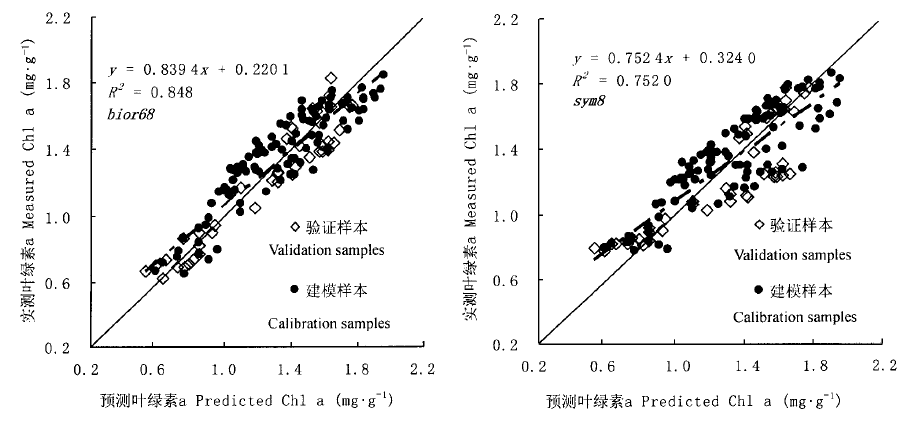
Fig.4 Relationship between multivariate regression based on wavelet-transformed soybean canopy spectral reflectance predicted chlorophyll a and measured chlorophyll a concentration
| [1] | Adams ML, Norvell WA, Peverly JH, Philpot WD (1993). Fluorescence and reflectance characteristics of Manganese deficient soybean leaves:effects of leaf age and choice of leaflet. Plant and Soil, 155/156, 235-238. |
| [2] | Bannari A, Morin D, Bonn F, Huete AR (1995). A review of vegetation indices. Remote Sensing Review, 13, 95-120. |
| [3] | Blackburn GA (1998). Spectral indices for estimating photosynthetic pigment concentrations:a test using senescent tree leaves. International Journal of Remote Sensing, 19, 657-675. |
| [4] | Bruce LM, Li J (2001). Wavelet for computationally efficient hyperspectral derivative analysis. IEEE Transactions on Geosciences and Remote Sensing, 39, 1540-1546. |
| [5] | Bruce LM, Koger CH, Li J (2002). Dimensionality reduction of hyperspectral data using discrete transform feature extraction. IEEE Transactions on Geosciences and Remote Sensing, 40, 2331-2338. |
| [6] | Chen J, Cihlar J (1996). Retrieving leaf area index of boreal conifer forests using Landsat TM images. Remote Sensing of Environment, 55, 153-162. |
| [7] | Gupta RK, Woolley JT (1971). Spectral properties of soybean leaves. Agronomy Journal, 63, 123-126. |
| [8] | Huang WJ (黄文江), Wang JH (王纪华), Liu LY (刘良云), Zhao CJ (赵春江), Song XY (宋晓宇), Ma ZH (马智宏) (2004). Correlation between grain quality indicators and spectral reflectance properties of wheat canopies by using hyperspectral data from winter wheat. Transactions of the Chinese Society of Agricultural Engineering (农业工程学报), 20, 203-207. (in Chinese with English abstract) |
| [9] | Huete AR (1988). A soil vegetation adjusted index (SAVI). Remote Sensing of Environment, 25, 295-309. |
| [10] | Jacquemoud S, Bacour C, Poilve H, Frangi JP (2000). Comparison of four radiative transfer models to simulate plant canopies reflectance:direct and inverse mode. Remote Sensing of Environment, 74, 417-481. |
| [11] | Lichtenthaler HK (1998). The stress concept in plants:an introduction. Annals of the New York Academy of Sciences, 851, 187-198. |
| [12] | Milton NM, Ager CM, Eiswerth BA, Power MS (1989). Arsenic- and Selenium-induced changes in spectral reflectance and morphology of soybean plants. Remote Sensing of Environment, 30, 263-269. |
| [13] | Myneni RB, Hall FG, Sellers PJ (1995). The interpretation of special vegetation indexes. IEEE Transactions on Geosciences and Remote Sensing, 33, 481-486. |
| [14] | Pu RL, Gong P (2004). Wavelet transform applied to EO-1 hyperspectral data for forest LAI and crown closure mapping. Remote Sensing of Environment, 91, 212-224. |
| [15] | Roujean JL, Breon FM (1995). Estimating PAR absorbed by vegetation from bidirectional reflectance measurements. Remote Sensing of Environment, 51, 375-384. |
| [16] | Rouse JW, Haas RH, Schell JA, Deering DW (1974). Monitoring the Vernal Advancements and Retrogradation of Natural Vegetation. NASA/GSFC, Final Report, Greenbelt, MD, USA, 1-137. |
| [17] | Song KS (宋开山), Zhang B (张柏), Li F (李方), Duan HT (段洪涛), Wang ZM (王宗明) (2005). Correlative analyses of hyperspectral reflectance, soybean LAI and aboveground biomass. Transactions of the Chinese Society of Agricultural Engineering (农业工程学报), 21, 36-40. (in Chinese with English abstract) |
| [18] | Wang D, Wilson C, Shannon M (2002). Interpretation of salinity and irrigation effects on soybean canopy reflectance in visible and near-infrared spectrum domain. International Journal of Remote Sensing, 23, 811-824. |
| [19] | Wang XZ (王秀珍), Huang JF (黄敬峰), Li YM (李云梅), Shen ZQ (沈掌泉), Wang RC (王人潮) (2002). Relationships between rice agricultural parameter and hyperspectral data. Journal of Zhejiang University (Agriculture & Life Sciences Edition) (浙江大学学报 (农业与生命科学版)), 28, 283-288. (in Chinese with English abstract) |
| [20] | Zhang XY (张兴义), Meng K (孟凯), Sui YY (隋跃宇) (1999). Change of stomatal resistance in soybean canopy at different nutritional level. System Sceinces and Comprehensive Studies in Agriculture (农业系统科学与综合研究), 15, 302-305. (in Chinese with English abstract) |
| [21] | Zhao CJ (赵春江), Huang WJ (黄文江), Wang JH (王纪华), Yang MH (杨敏华), Xue XZ (薛绪掌) (2002). Studies on the red edge parameters of spectrum in winter wheat under different varieties, fertilizer and water treatments. Scientia Agricultura Sinica (中国农业科学), 35, 980-987. (in Chinese with English abstract) |
| [1] | WU Han, BAI Jie, LI Jun-Li, Guli JIAPAER, BAO An-Ming. Study of spatio-temporal variation in fractional vegetation cover and its influencing factors in Xinjiang, China [J]. Chin J Plant Ecol, 2024, 48(1): 41-55. |
| [2] | LI An-Yan, HUANG Xian-Fei, TIAN Yuan-Bin, DONG Ji-Xing, ZHENG Fei-Fei, XIA Pin-Hua. Chlorophyll a variation and its driving factors during phase shift from macrophyte- to phytoplankton-dominated states in Caohai Lake, Guizhou, China [J]. Chin J Plant Ecol, 2023, 47(8): 1171-1181. |
| [3] | CHEN Xue-Ping, ZHAO Xue-Yong, ZHANG Jing, WANG Rui-Xiong, LU Jian-Nan. Variation of NDVI spatio-temporal characteristics and its driving factors based on geodetector model in Horqin Sandy Land, China [J]. Chin J Plant Ecol, 2023, 47(8): 1082-1093. |
| [4] | MIAO Li-Juan, ZHANG Yu-Yang, CHUAI Xiao-Wei, BAO Gang, HE Yu, ZHU Jing-Wen. Effects of climatic factors and their time-lag on grassland NDVI in Asian drylands [J]. Chin J Plant Ecol, 2023, 47(10): 1375-1385. |
| [5] | ZHU Yu-Ying, ZHANG Hua-Min, DING Ming-Jun, YU Zi-Ping. Changes of vegetation greenness and its response to drought-wet variation on the Qingzang Plateau [J]. Chin J Plant Ecol, 2023, 47(1): 51-64. |
| [6] | WEN Ke, YAO Huan-Mei, GONG Zhu-Qing, NA Ze-Lin, WEI Yi-Ming, HUANG Yi, CHEN Hua-Quan, LIAO Peng-Ren, TANG Li-Ping. Influence of inundation frequency change on enhanced vegetation index of wetland vegetation in Poyang Lake, China [J]. Chin J Plant Ecol, 2022, 46(2): 148-161. |
| [7] | YUAN Yuan, MU Yan-Mei, DENG Yu-Jie, LI Xin-Hao, JIANG Xiao-Yan, GAO Sheng-Jie, ZHA Tian- Shan, JIA Xin. Effects of land cover and phenology changes on the gross primary productivity in an Artemisia ordosica shrubland [J]. Chin J Plant Ecol, 2022, 46(2): 162-175. |
| [8] | YAN Zheng-Bing, LIU Shu-Wen, WU Jin. Hyperspectral remote sensing of plant functional traits: monitoring techniques and future advances [J]. Chin J Plant Ecol, 2022, 46(10): 1151-1166. |
| [9] | Ning LIU, Shou-Zhang PENG, Yun-Ming CHEN. Temporal effects of climate factors on vegetation growth on the Qingzang Plateau, China [J]. Chin J Plant Ecol, 2022, 46(1): 18-26. |
| [10] | NI Ming, ZHANG Xi-Yue, JIANG Chao, WANG He-Song. Responses of vegetation to extreme climate events in southwestern China [J]. Chin J Plant Ecol, 2021, 45(6): 626-640. |
| [11] | JI Yu-He, ZHOU Guang-Sheng, WANG Shu-Dong, WANG Li-Xia, ZHOU Meng-Zi. Evolution characteristics and its driving forces analysis of vegetation ecological quality in Qinling Mountains region from 2000 to 2019 [J]. Chin J Plant Ecol, 2021, 45(6): 617-625. |
| [12] | CHEN Zhe, WANG Hao, WANG Jin-Zhou, SHI Hui-Jin, LIU Hui-Ying, HE Jin-Sheng. Estimation on seasonal dynamics of alpine grassland aboveground biomass using phenology camera-derived NDVI [J]. Chin J Plant Ecol, 2021, 45(5): 487-495. |
| [13] | ZHOU Ming-Xing, LI Deng-Qiu, ZOU Jian-Jun. Vegetation change of giant panda habitats in Qionglai Mountains through dense Landsat Data [J]. Chin J Plant Ecol, 2021, 45(4): 355-369. |
| [14] | XU Guang-Lai, LI Ai-Juan, XU Xiao-Hua, YANG Xian-Cheng, YANG Qiang-Qiang. NDVIdynamics and driving climatic factors in the Protected Zones for Ecological Functions in China [J]. Chin J Plant Ecol, 2021, 45(3): 213-223. |
| [15] | GUO Qing-Hua, HU Tian-Yu, MA Qin, XU Ke-Xin, YANG Qiu-Li, SUN Qian-Hui, LI Yu-Mei, SU Yan-Jun. Advances for the new remote sensing technology in ecosystem ecology research [J]. Chin J Plant Ecol, 2020, 44(4): 418-435. |
| Viewed | ||||||
|
Full text |
|
|||||
|
Abstract |
|
|||||
Copyright © 2022 Chinese Journal of Plant Ecology
Tel: 010-62836134, 62836138, E-mail: apes@ibcas.ac.cn, cjpe@ibcas.ac.cn